Last updated: 2023-01-04
Run chromRegions()
chromRegions() takes a file with the sizes of the chromosomes and draws a ggplot2-based bar plot. Then takes a list of regions in a BED-like format to draw them into each chromosome. The inputs chrom.sizes and regions can be supplied as a list of character with path to the file where the information is stored or a list of data frame.
Required input
The crhom_sizes input is:
chrom_sizes = "../testdata/mm10.chrom.sizes"
chrom_sizes %>% read.delim(header = F) %>% head()
## V1 V2
## 1 1 195471971
## 2 10 130694993
## 3 11 122082543
## 4 12 120129022
## 5 13 120421639
## 6 14 124902244The regions_list is a list of characters or dataframes. It can have as many elements as wanted and it has the following structure:
regions_list <- list("Regions1" = "../testdata/mm10.regions.tsv",
                     "Regions2" = "../testdata/mm10.regions2.tsv",
                     "Regions3" = "../testdata/mm10.regions3.tsv")
regions_list[[1]] %>% read.delim(header = F) %>% head()
## V1 V2 V3 V4 V5 V6
## 1 1 57348975 57377520 region2 28545 -
## 2 1 91403055 91406029 region4 2974 -
## 3 1 92992344 92997067 region6 4723 -
## 4 1 125174891 125177979 region10 3088 +
## 5 10 18796805 18831930 region18 35125 -
## 6 10 20310505 20312760 region19 2255 -Default run
The default run requires only the chrom_sizes and the regions arguments, either as a path to a file or a data frame.
chromRegions(chrom_sizes = "../testdata/mm10.chrom.sizes", regions_list = regions_list)
# Read the data
chrom_sizes = "../testdata/mm10.chrom.sizes"%>% read.delim(header = F)
regions = regions_list %>% purrr::map(~read.delim(.x, header = F))

chromRegions(chrom_sizes = chrom_sizes, regions_list = regions)
Chromosome order
chromRegions(chrom_sizes  = "../testdata/mm10.chrom.sizes",
             regions_list = regions_list,
             chr_order    = c(1,3,4,2,5,6,7,9,8,19,11,10,12,13,15,14,16,17,18,"X","Y","M", "MT") )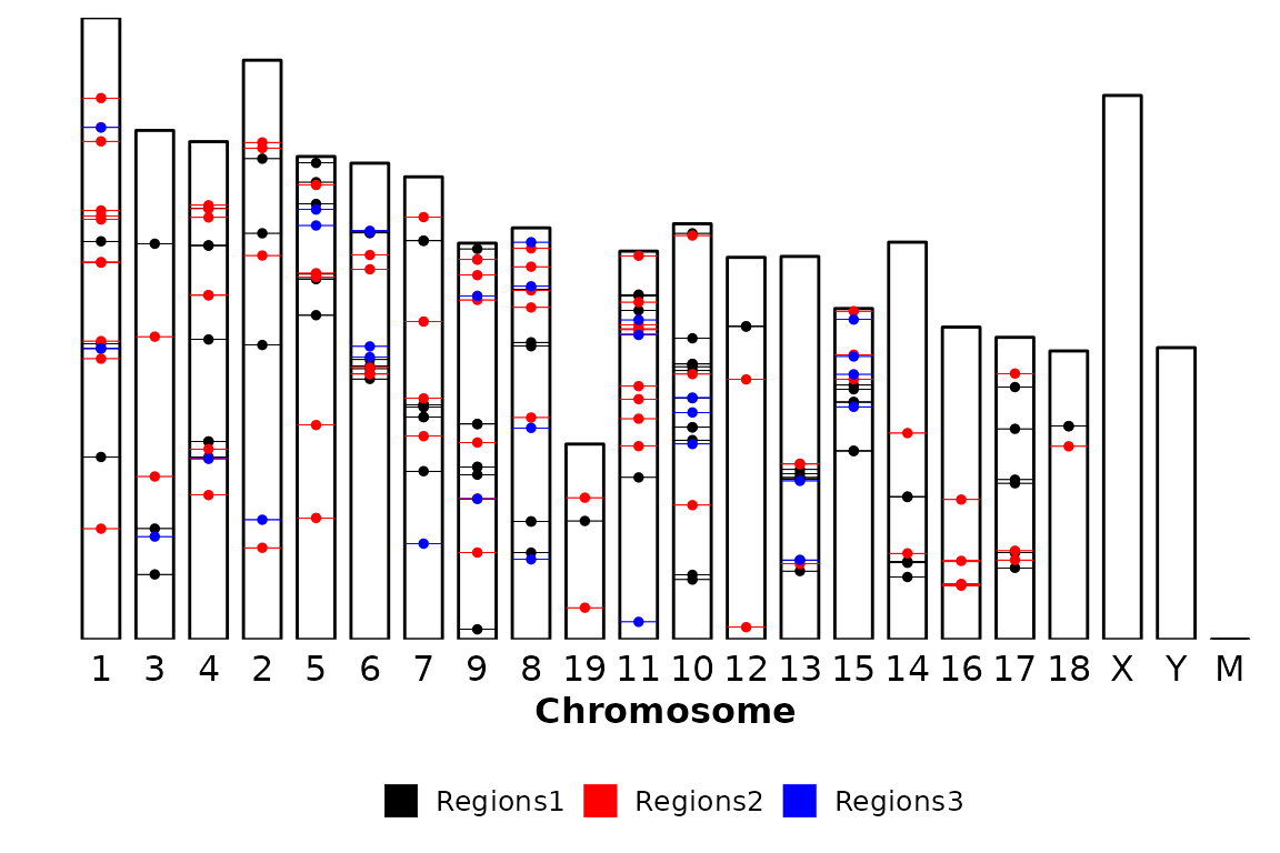
Exclude chromosomes
Very often, the genome assemblies of a lot of species have chromosomes/scaffolds with strange names, which are not nice to plot. These can be excluded using the chr_exlude argument with a vector of regular expressions that match the chromosomes to exclude. By default chr_exclude removes the most usuall strange chromosomes, but if you want to remove more chromosomes or don’t want to remove any, you can change the chr_exclude argument.
An example that excludes all the chromosomes that contain a dot in the name:
chromRegions(chrom_sizes  = "../testdata/mm10.chrom.sizes",
             regions_list = regions_list,
             chr_exclude  = c("\\."))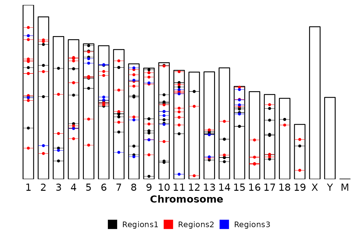
Here you have an example that does not remove any chromosome.
chromRegions(chrom_sizes = "../testdata/mm10.chrom.sizes",
regions_list = regions_list,
chr_exclude = c(" "))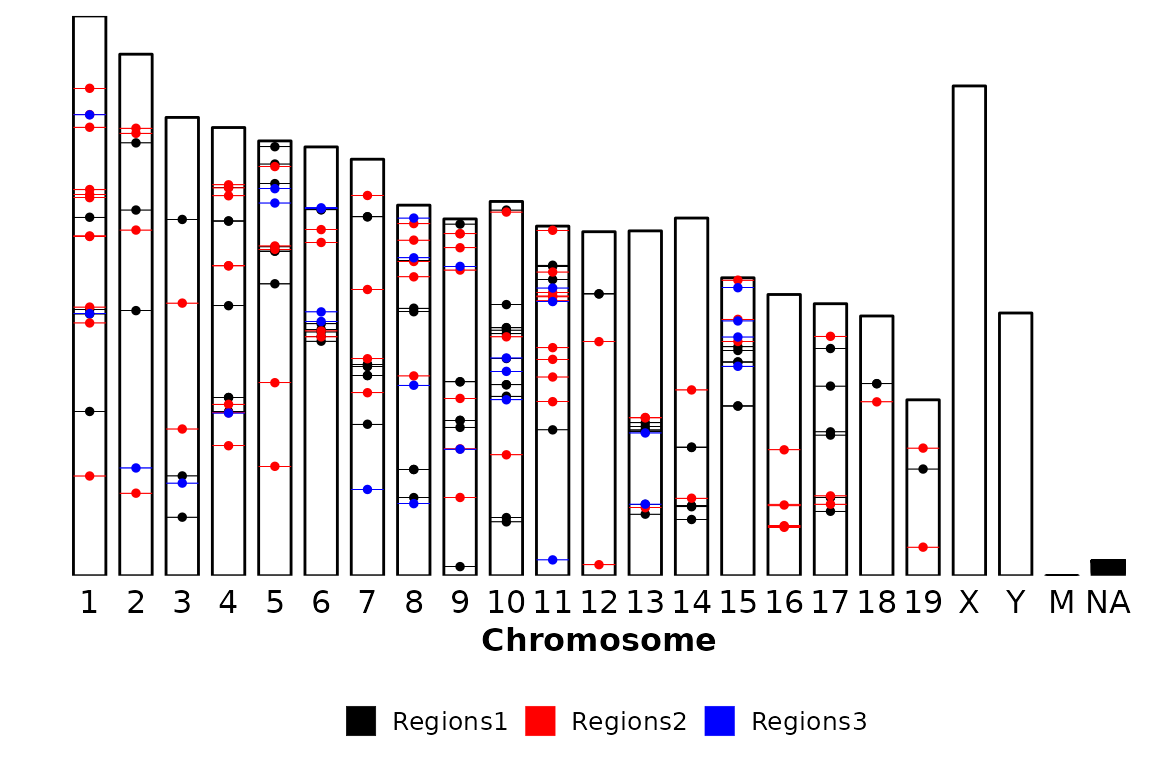 Note that, since we are converting the chromosome names to an ordered factor with
 chr_order, the chromosome names that do not appear in chr_order will be groupped and plotted into a NA category.
Customization
Flip axes
chromRegions() allows flipping the axes by setting the coord_flip argument to TRUE.
chromRegions(chrom_sizes  = "../testdata/mm10.chrom.sizes",
             regions_list = regions_list,
             coord_flip   = T)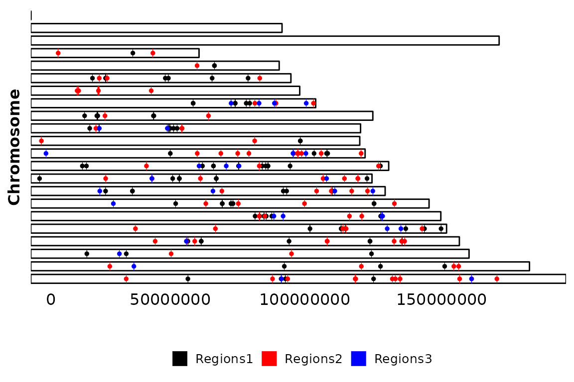
Draw the points
By default, chromRegions() draws a line/rectangle and a point in the middle of each region. To avoid drawing the points, the argument draw_points can be set to FALSE.
chromRegions(chrom_sizes  = "../testdata/mm10.chrom.sizes",
             regions_list = regions_list,
             draw_points  = F)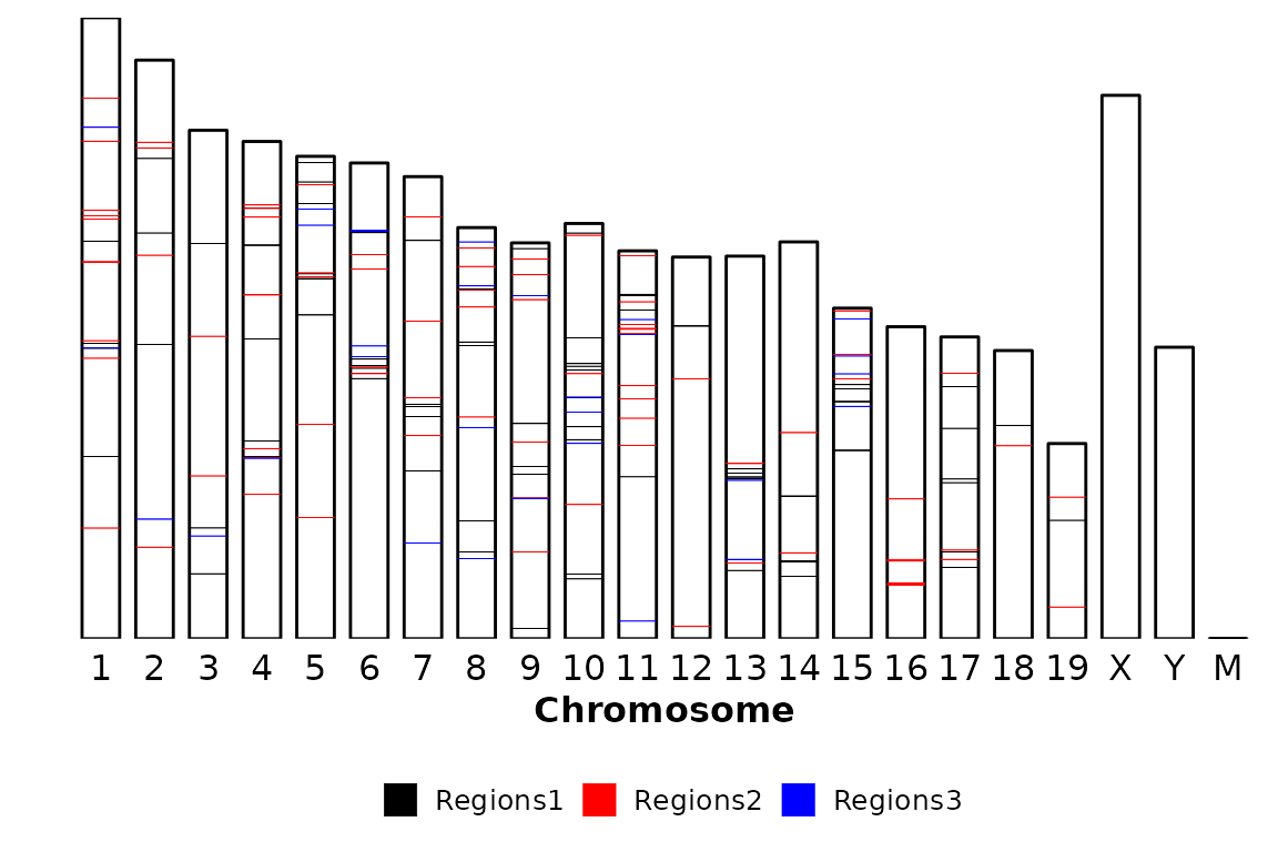
Color
By default, the regions are colored by region (i.e. each element in regions_list). This can be controlled with the colors argument, which accepts a character vector with valid color names and the same length as regions_list
chromRegions(chrom_sizes = "../testdata/mm10.chrom.sizes",
regions_list = regions_list,
colors = c("Black", "Yellow", "Green"))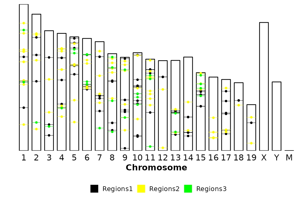 If you want to color by strand, just turn
 color_by to "strand".
chromRegions(chrom_sizes   = "../testdata/mm10.chrom.sizes",
             regions_list  = regions_list,
             colors        = c("Darkgreen", "Darkred"),
             color_by      = "strand")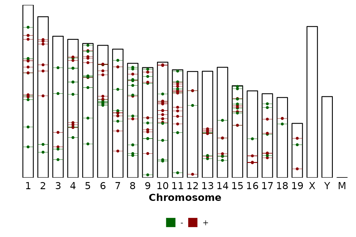
Now, imagine that we have regions that do not have a defined strand (e.g. most ChIP-seq peaks). In this case, the color_by is internally converted to "region" and the regions are colored by region set (i.e. elements in regions_list). Look at this example with only one region set whose strand values are converted to “.”.
# Read and format regions file to have strand as "."
regions_no_strand <- list("Regions1" = read.delim("../testdata/mm10.regions.tsv", header = F) %>% dplyr::mutate(V6 = "."))

# Draw the plot
chromRegions(chrom_sizes   = "../testdata/mm10.chrom.sizes",
             regions_list  = regions_no_strand,
             color_by      = "strand",
             colors        = c("Gold3", "Darkgreen"))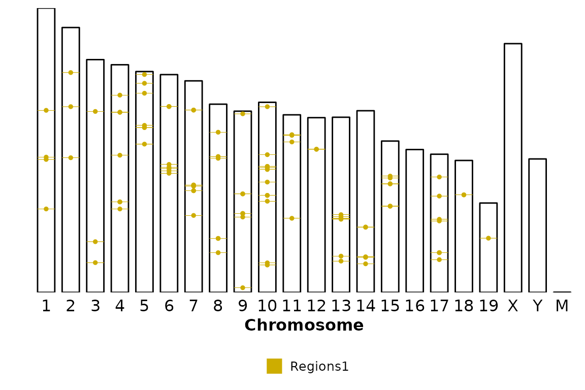
Titles
Title and subtitle can be supplied through the arguments title and subtitle, respectively. By default, they are set to NULL, but can accept a character of length 1.
chromRegions(chrom_sizes   = "../testdata/mm10.chrom.sizes",
             regions_list  = regions_list,
             title         = "This is a title",
             subtitle      = "This is a subtitle")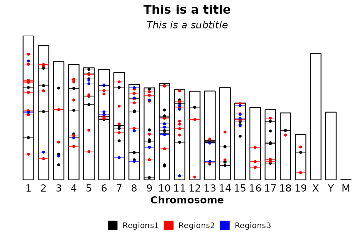
Also, the labels of the axes can be set or removed through the xlab and ylab arguments. By default, the X axis label is set to “Chromosome” and the Y axis is set to "", but they can be removed setting the corresponding arguments to NULL or changed to any value.
chromRegions(chrom_sizes = "../testdata/mm10.chrom.sizes",
regions_list = regions_list,
xlab = NULL,
ylab = "Position in the chromosome")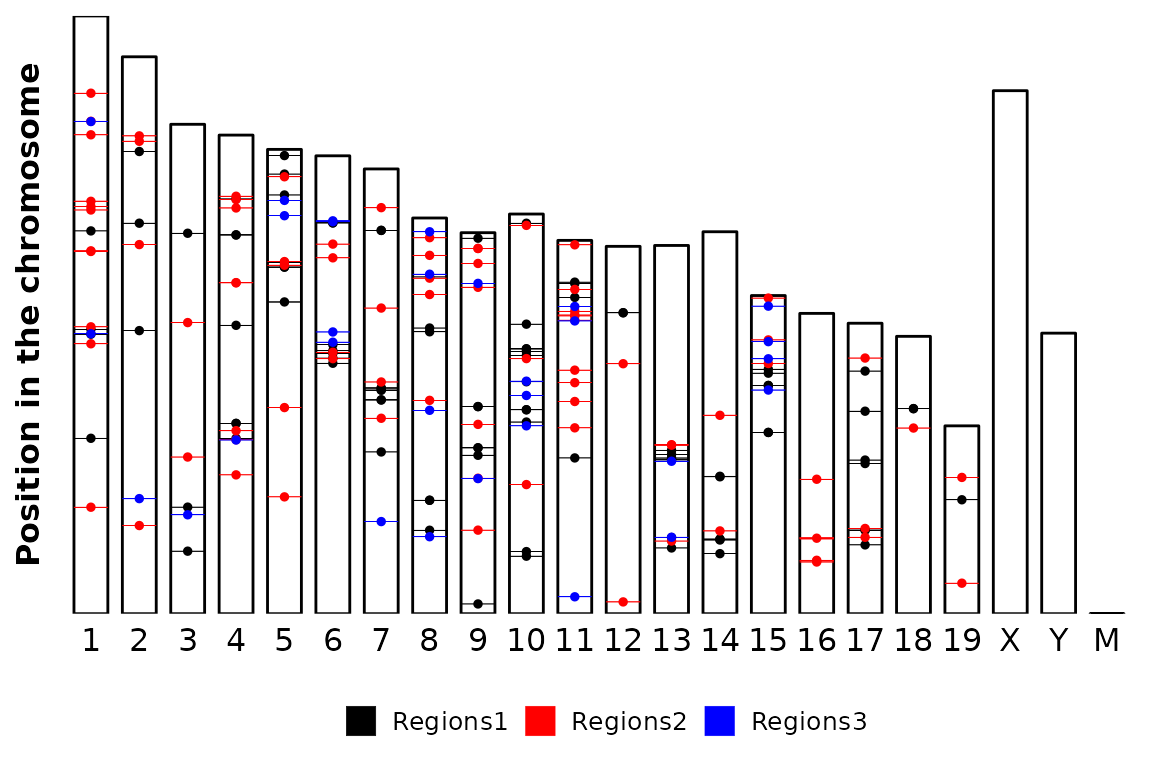 Finally, a caption can be included in the bottom-right corner by setting the
 caption argument. By default, caption is set to NULL and it can be set to TRUE or any character. If caption is set to a character, whatever is written will be placed in the bottom-right corner. Instead, if it is set to TRUE, what will be written will be the number of regions in the input region sets.
Here there is an example with any character:
chromRegions(chrom_sizes   = "../testdata/mm10.chrom.sizes",
             regions_list  = regions_list,
             caption       = "This is a caption")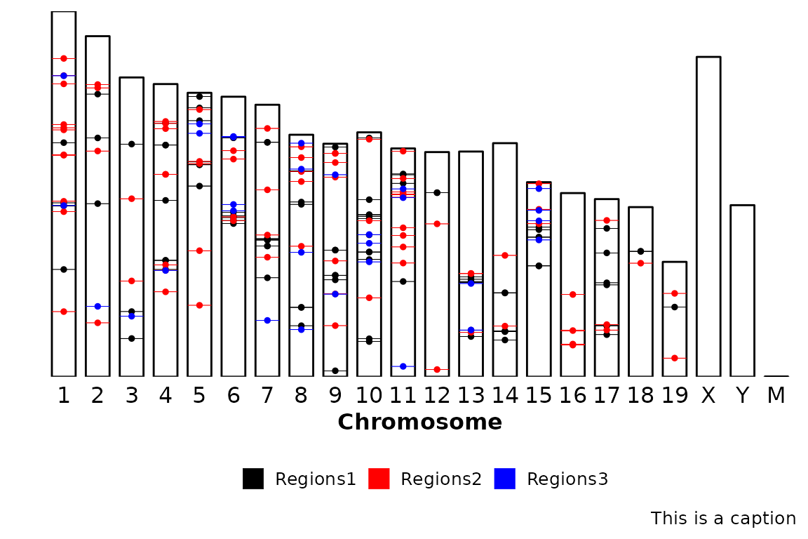
On the other hand, if caption is set to TRUE, the caption will show the number of regions in the input regions set (regions).
chromRegions(chrom_sizes   = "../testdata/mm10.chrom.sizes",
             regions_list  = regions_list,
             caption       = TRUE)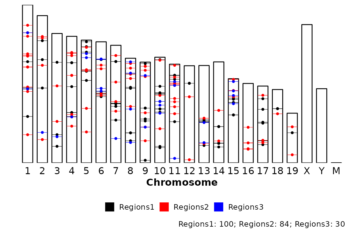
Legend
The position of the legend is, by default, the bottom of the plot. This can be changed by changing the legend argument to one of “bottom”, “right”, “top”, “left” or “none” (no legend). The legend argument is passed through ggpubr::theme_pubr().
chromRegions(chrom_sizes   = "../testdata/mm10.chrom.sizes",
             regions_list  = regions_list,
             legend        = "right")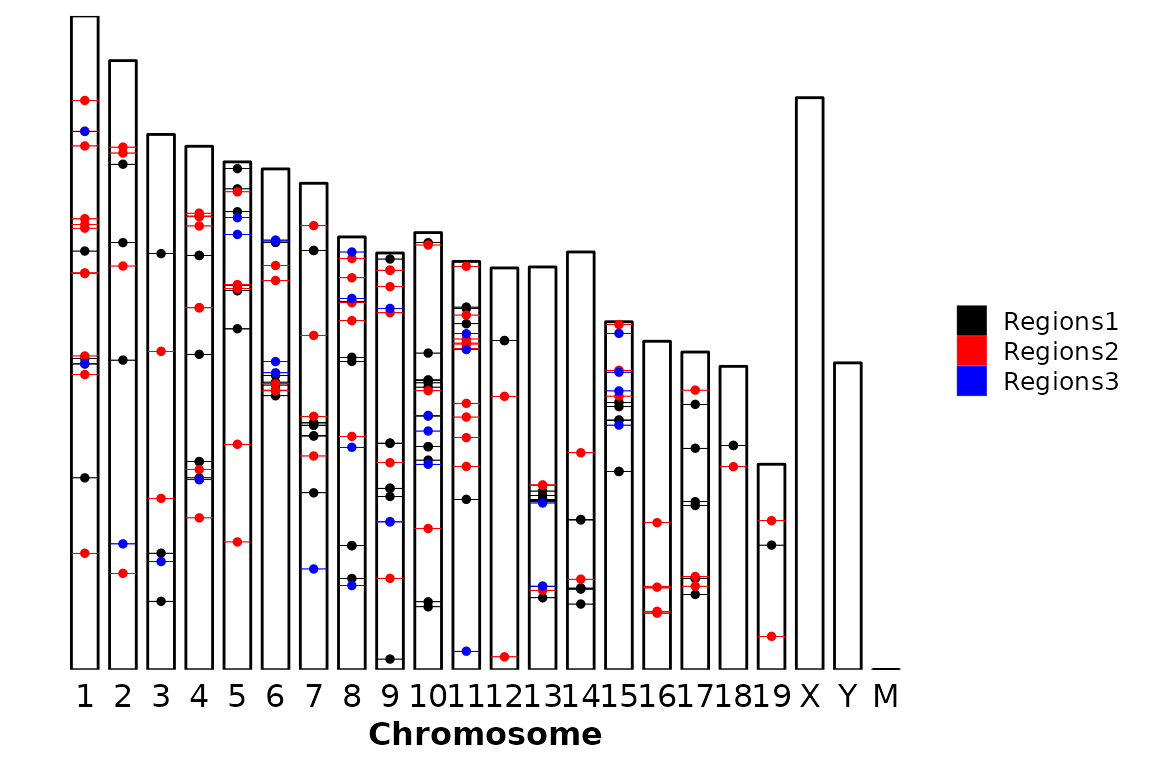
chromRegions(chrom_sizes = "../testdata/mm10.chrom.sizes",
regions_list = regions_list,
legend = "none")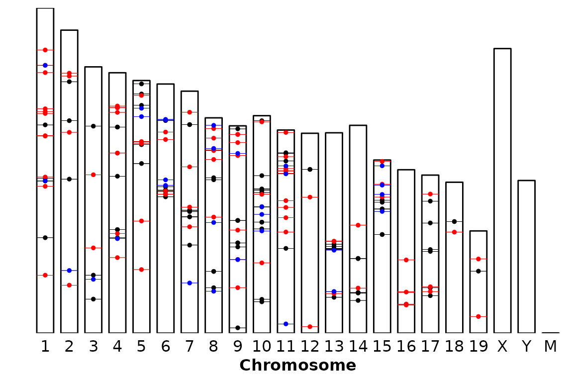 ### Y axis
By default, the Y axis is not plotted, which means that the y_text_size is set to NULL. However, it can be plotted by setting the size_y_text argument to a number which will be used as size of the text in the Y axis.
chromRegions(chrom_sizes   = "../testdata/mm10.chrom.sizes",
             regions_list  = regions_list,
             y_text_size   =  10)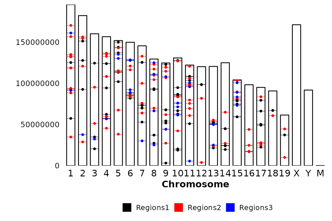
Further costumization
Since chromRegions() outputs a ggplot2-based bar plot, it can be further customized like any other ggplot2-based plot.